Conditionally format rows in Excel depending on date range
Sometimes I get asked Excel questions. This is one of those times!
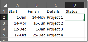
Given a spreadsheet with rows that contain a start and finish date, format the rows in the past, present and future in different colours, so that it looks like this:

I initially tried using a formula with Excel’s Conditional Formatting feature. Despite this being the recommended solution in some search results, I just found it set the one format for all the rows – not what I wanted. This post by Joseph D’Emanuele put me on the right track.
Here’s what I ended up doing:
- Add a new column next to your existing data
- In the first cell of this new column, insert the formula
=IF(B2 < TODAY(), "Past", IF(A2 > TODAY(), "Future", "Current")) - Copy this formula down to the remaining rows. eg.
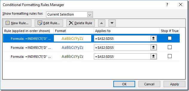
- Now select all the rows you want to format (for me that’s A2:D5)
- On the Home menu tab, select Conditional Formatting, then Manage Rules
- You will add 3 rules – one for each status.
- Click New Rule
- Select Use a formula to determine which cells to format
- In Format values where this formula is true, enter =INDIRECT(“D” &ROW()) = “Future”
- Click Format and choose the desired formatting to apply for Future dates
- Click OK and repeat adding new rules for “Current” and “Past”
- You should end up with something like this:
- Click OK and you should have rows formatted different colours depending on whether the start/finish date is in the past, current or in the future!
- You can optionally choose to hide the Status row if you’d rather not see it all the time.

Note that the formula in the conditional formatting (=INDIRECT(“D” &ROW()) = “Future”) is hard-coded to the column – “D” in my case. If you move data around, you’ll need to update this to refer to the new column letter.